Building a Neural Network to predict the next best pass in a football match

So what was my idea? It’s almost certainly been done before, but could I create a neural network that predicted the likely next best pass in a football match? This clearly wouldn’t be complex enough for production use cases, but you can see how one that is complex enough might be useful to evaluate player performance or even be used as the AI in a video game!

Building the Neural Network

Where do you start when it comes to training a neural network?

1. What do you want to predict?
2. What data do you have to make those predictions on?

I wanted to predict the next next best pass in a football match and in order to do that, I needed some data on where the ball was, who was in possession of it and where everyone was on the pitch. I discovered some data by SkillCorner that included data for 10 matches from the Australian A-League. The data essentially consisted of events data (when passes were made, etc.) and positioning data (where players are on the pitch at each frame).

With data available, I could focus on the three main elements of any neural network.

1. How do I structure my inputs for training (and therefore inference)?
2. How do I structure my outputs? Do I want a single value or a distribution?
3. What do I put between the input and output to train a network of sufficient complexity to model my scenario generically?

Design

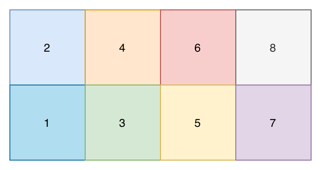
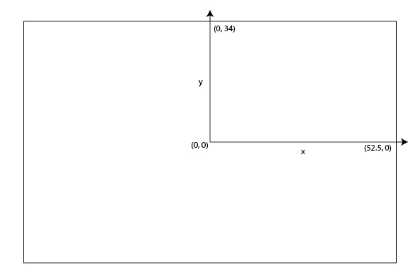
The core of my neural network design centred around the input shape. I didn’t want to create a complex input shape of the x and y position of every player on that pitch, because that seemed quite complex (though probably what you’d do if creating a model for real). Instead I opted for a model where the pitch is split up into 8 zones, and the input is the number of players (split on attacking and defending team) in each zone, and the zone that the ball is in.

Input Shape

An example input into the network would therefore look something like the below. The first number is the zone the ball is in, and each subsequent pair of numbers contains the number of attacking and defending players in that zone. Zone 1 is relative and is the attacking teams right back position

In fact, one of the most challenging parts of this project was parsing the data out of the training datasets and getting it into the right structure for the neural network!

There are other data preparation tasks you'd likely perform in preparing data for a neural network such as normalisation, but given this was a purely educational activity, I haven't. 

Regarding the output shape, the main question on my mind was do I predict the zone directly (i.e. 2 or 7), or do I output a probability distribution across all zones. I decided on the latter as it would better demonstrate the neural networks ability to “learn”.

Output Shape

The output therefore looks like the below. The probability across all 8 zones adds up to to 1.

Designing the input and output shapes came somewhat naturally. At no point however did the design of the hidden layers of the neural network come naturally. In fact, it was purely based on experimentation. Well, I tested one approach and it seemed to work so I left it alone!

Layers

The idea of a neural network is that by ‘massaging’ weights and biases (parameters) in-between the input and output layer, you can find a configuration that results in accurate outputs. Feeding all inputs into one neuron with a single weight is unlikely to have enough complexity to model our problem. Equally, one with trillions of parameters is probably not economically viable to train and / or add much accuracy. However, it turns out if you connect each input to 8 neuron’s which then feed the output layer, you can create model that’s somewhat accurate (at least, the next best pass is generally plausible!)

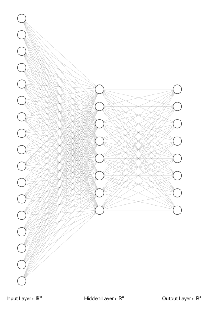
As a result of this design, there are 216 trainable parameters.

	Weights	Biases	Total Parameters
Dense 1 (Hidden Layer)	136	8	144
Dense 2 (Output Layer)	64	8	72
Total	200	16	216

Whilst not an exact comparison, large language models such as those provided by ChatGPT container trillions of parameters. Given much of the computational cost of models comes from training them, being able to achieve better accuracy per parameter is a key innovation area of neural networks.

Determining the structure of the neural network also requires you to choose activation methods for the neuron’s. In addition to ReLU, the softmax activation function which takes the outputs of the final hidden layer and returns a probability distribution across the output (zones). You’ll see softmax outputs in many categorisation models such as topic and sentiment detection. There’s not much on activation methods here as that’s my next area of study.

Implementation

Implementation of the neural network consists of a couple of stages:

1. Transforming data and organising it (splitting it in training and validation sets)
2. Creating the network structure (i.e. the layers and their configurations)
3. Training the network

Thankfully, steps 2 and 3 are made incredibly simple by using frameworks such as TensorFlow.

Training

The SkillCorner dataset contains 10 football matches, with event and positioning data. Across 6 matches (I could have done all 10, but didn’t… for some reason!). The transformation step was essentially to look for each passing option event and for that event, find the positions of all the players on the pitch at that point in time. This resulted in 3680 passing scenarios where I could extract the features (the position of the players and the ball) and the labels (the zone that the pass was actually made to).

The network is initially created, with the relevant layers added to it (as discussed in the design). Finally, the fit method is called which takes in the features and labels and trains the parameters.

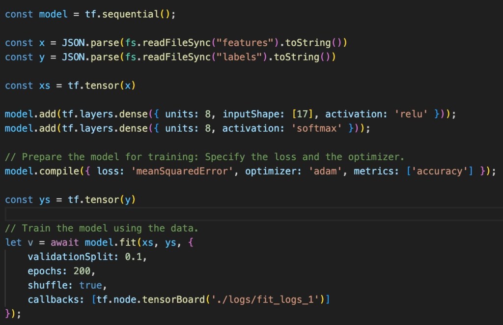
The compile method introduces 2 important elements of the training process, the loss and optimisation functions. Both elements are explained in my previous blog and so I won’t repeat that here. But to summarise, the loss function tells the training process how far it is from being accurate (according to the training data) and the optimiser is the thing that ‘massages’ the parameters in such a way that reduces the model loss (a process known as backpropagation).

Two other parameters of interest are the validationSplit and epoch. A validationSplit helps test for overfitting; if the model can predict really well for its training data but is awful on inputs it’s never seen before, it’s said to be overfitted. Overfitting can happen when too many epochs are ran over a given amount of data. An epoch is a run through all the training data alongside the relevant optimisations; do this too many times on a small (relative to model complexity) amount of data and the model will be overfitted.

The diagram below shows the output of the loss function for each epoch. You want the loss to decrease to as close to 0 as possible.

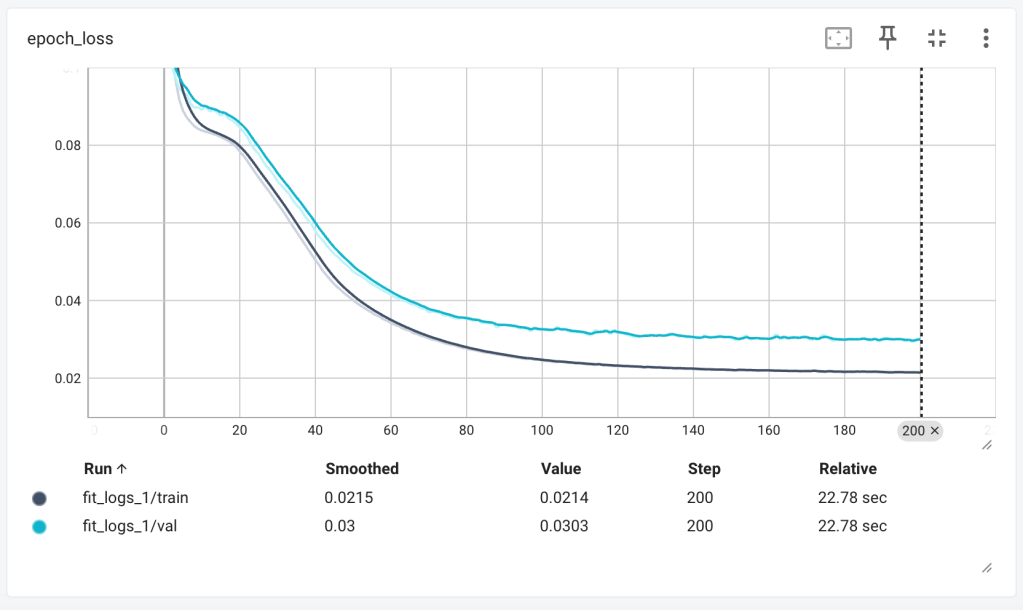
As loss decreases, you’d expect accuracy to increase, which is exactly what we see. In both the loss and accuracy graphs, we can see the lull in performance between 10 and 20 epochs – I believe this is the optimiser finding its way out of local minima, where it believes it’s found the best parameter values and decreases the learning rate, only to find better solutions do exist.

The result of the training process is a set of ‘massaged’ numbers. The image below shows the trained weights of the first dense layer, containing 136 weights (the biases aren’t shown below).

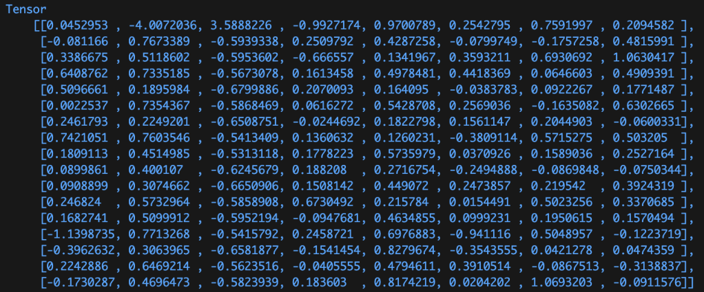
When a model is packaged up and distributed for use, it’s these weights and biases that are worth millions of dollars and worth protecting. Whilst some models are open-sourced (and therefore these values are visible), others aren’t and their structure and parameter values are kept secret.

Environmental Considerations

Notices how across both graphs above, the model performance ‘flattens’ out after around 100 epochs. Running an epoch is a computationally intensive process (for complex models) and as such, knowing how many epochs are suitable for the model can help decrease the costs of training runs. Cost both in terms of money, but also energy required.

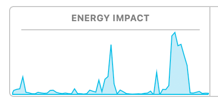
Training the LLMs we all use today takes on the order of terrajoules (trillions of joules). Something close to the amount of energy released in the atomic bomb dropped in Hiroshima. It would take a residential solar panel around 400 years to generate that much electrical energy. How much energy usage warrants the value provided by these models? Or perhaps more importantly, what methods of electrical energy generation are worth the value of these models? Fossil, Nuclear, Renewable?

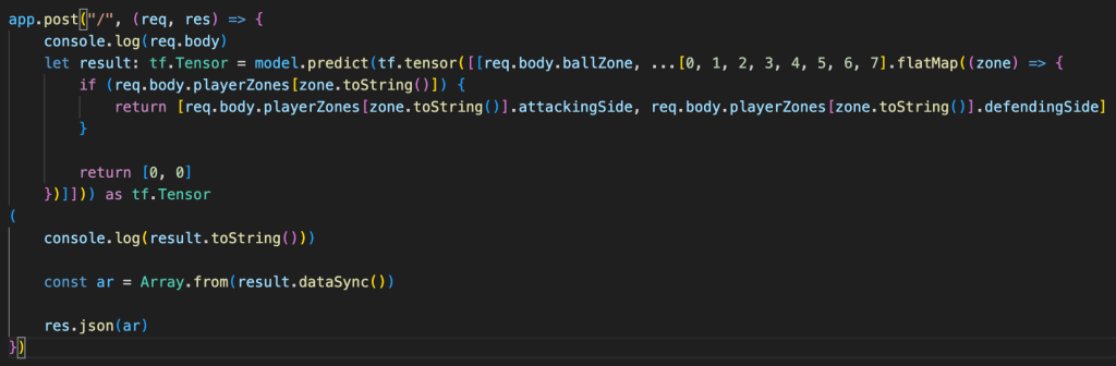
Inference

Now that we have a trained model, we can send it some data it probably hasn’t seen before (in the structure of the input shape) and get back a probability distribution of the best next passing zone. In my experimentation, I hosted my model behind a simple API, much like ChatGPT.

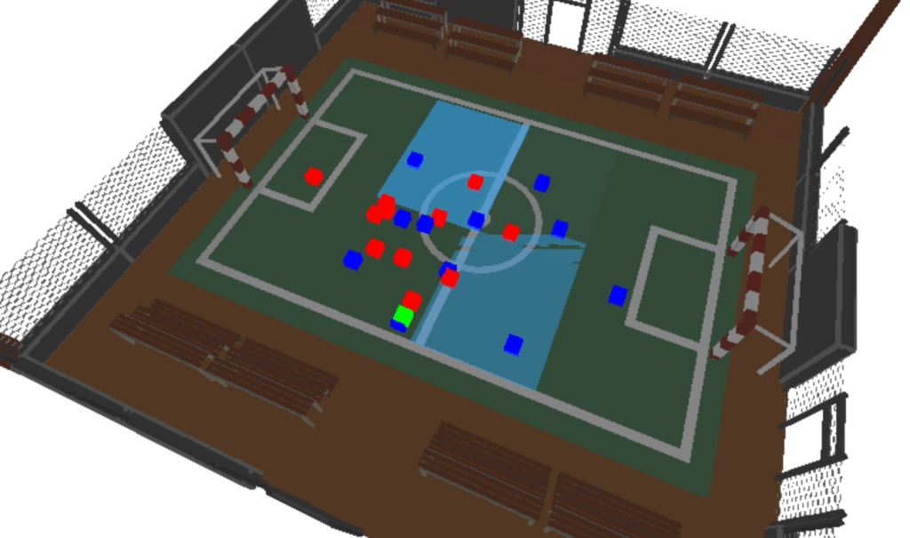
Visualisation

But that’d be an anti-climax of a blog!… I’m a massive fan of three.js, I’ve used it in previous blogs and find it’s a fantastic, easy to use method of visualising computational processes. The screenshot below and video at the top of this blog visualise one of the football matches in the SkillCorner dataset, overlayed with rectangles of varying opacity based on the models pass prediction response by zone. Pretty cool!

What Next?

The best part of any project is the ideas it gives you on where to take your studies next. For me that’s diving a bit deeper into neural networking concepts such as optimisation methods and activation functions. It also includes continuing by studies of Large Language Models, for which neural networks play a critical part.

Additionally, my role as a Software Engineer isn’t that of training any sort of Machine Learning models; I deploy them and utilise them within my applications. So how much do I need to know about this technology to do that well? I relate it back to understanding how transistors build up to create logic gates, that create Arithmetic Logic Units (ALUs) that create Central Processing Units (CPUs); I don’t directly apply this knowledge day-to-day, but it’s always in the back of my mind, validating decisions and ensuring I write performant and reliable code.

Finally, sports provide an exciting opportunity to learn more about statistical methods and Machine Learning techniques. With the open source data available to apply that learning, I can see myself getting lost in this area throughout 2026. I’ve just bought Soccermatics and can’t wait to get stuck into it.