Today, the sales pitch isn’t Digital, it’s Data; Data-driven, data as a first class citizen, data powered… This post aims to cut through the smoke and mirrors to reveal what’s behind the sales pitch, breaking down the key building blocks of any Data Analytics platform through a worked example following a fictions e-commerce organisation, Congo, on their journey to data driven insights… ok, I’m partial to a strap-line also!
This post focusses on native AWS Data Analytics services – as such, if you’re studying for your AWS Data Analytics Speciality, I hope this post can help you achieve that goal. Alternatively, if you’re just here out of curiosity, thank you for taking the time to read.

Congo.co.uk
Our customer, Congo… runs an online store that sells a wide range of products. The store runs on a number of key IT systems (known as operational systems) such as the Customer Relationship Management (CRM) system, the Order and Product Management systems and of course, the website.
Congo are sitting on years worth of customer and order information that they want to make use of to better serve their customers. They understand trends can be short-lived and seemingly random (i.e. the chessboard following the release of The Queen’s Gambit), whilst others are more seasonal (paddling pools over the summer). Further to this, trends vary across the globe (those in northern Canada probably aren’t a fan of outdoor paddling pools!). Congo believe that analysing this information can improve the customer experience and increase sales, an hypothesis that can be tested using Data Analytics.
What is Data Analytics
The end goal of any Data Analytics process is to inform a decision – the decision may be made by the analytics platform itself (i.e. a betting analytics platform might automatically change odds based on the result of some analytics) or by a human who is supported by the analytics. Where humans are involved, often the analytics platform must have a way of presenting information for human consumption – this is known as visualisation.
In Congo’s case, they hope that the analytics platform can make the decisions as to what products are ‘hot’ and for that information to be fed to their website automatically. However, they would also like dashboards showing them what impact these decisions are having on sales.
The initial design by the Congo IT team was to directly query the operational systems; however, they quickly encountered problems:
- Whenever analytical queries are executed, the database saturates and customers are left reporting error messages on the online store.
- Writing software to join the results of queries from multiple database technologies is challenging and error prone.
- The process is very reactive – whilst this is fine for querying vast amounts of historic data, it’s slow when wanting to understand what’s happening right now (i.e. what products are being sold right now).
In short, due to the amount of data and questions being asked of it, the current IT isn’t capable of answering these questions whilst also supporting day-to-day operations such as allowing customers to purchase products. When an organisation finds themselves in this situation, the solution is typically to deploy a Data Analytics platform.
A Data Analytics platform must often solve for the following core problems:
- The data doesn’t fit on a single computer.
- Even if the data did fit on a single computer, the resources available (CPU, memory, IO, etc.) are not able to perform the analytics in an acceptable timeframe.
These issues typically mean that analytical platforms require many computers to work together, a technique known as Distributed Computing.
Distributed Computing for Data Analytics
Let’s assume we wanted to count the number of words in the dictionary – if I sat down and counted 1 word every second, it would take me a couple of days to come up with the answer. How can I speed this process up? If I split the dictionary into 3 equal pieces and found 3 friends to help (I’ve no idea what friend would help another do this…), I could count the number of words in the dictionary in a day. We’d each calculate how many words are in 1/3 of the dictionary (importantly, at the same time) and then at the end come together and sum the individual counts. This is the core concept behind distributed computing for data analytics.
When dealing with extremely large volumes of data, we need ways of splitting it up such as:
- Spreading the data across a number of computers. For example, splitting a text file every 10 lines and sending each set of lines to a different computer, and
- Reducing the amount of data that needs to be queried. For example, if looking for an electrician, you don’t scan through a list of all electricians in your country, you scan through those that are in your city. Any way that we can reduce the amount of data that needs to be queried can only improve the speed at which we can perform the analysis.
To introduce the concept of distributing data across many computers, we’ll consider two techniques:
- Partitioning – to split data into an unbounded number logical chunks (i.e. I might partition on year, city, etc.)
- Clustering – split data into a defined number of buckets whereby based on some algorithm, we know which bucket our required data is in.
In Congo’s case, to understand the longer term trends, they need to analyse a vast amount of historical data (terabytes) across 2 datasets to understand the number of products sold per year, per city, aggregated by product type (i.e. we sold 812,476 paddling pools in London in 2020). The 2 datasets involved are:
- An Order table, and
- A Product table containing reference data such as the product name, RRP, etc.
Querying this quantity of data on a single computer isn’t feasible due to the amount of time the query would take to run. As such, we need to use the 2 techniques mentioned to split the datasets so that they can be distributed amongst a number of computers.
The table below is an example of the Order table showing the PRODUCT_ID column which is a value we can use to look up product details in the Product table (i.e. I’ll be able to find PRODUCT_ID 111 in the Product table).
| ROW_NO | NAME | CITY | YEAR | PRODUCT_ID |
|---|---|---|---|---|
| 1 | SIMON | LONDON | 2020 | 111 |
| 2 | JANE | YORK | 2019 | 897 |
| 3 | SIMON | BRIGHTON | 2020 | 298 |
| 4 | SIMON | LONDON | 2019 | 61 |
| 5 | SARAH | LONDON | 2020 | 111 |
As our queries are based on individual years and cities, we can start by partitioning the data on these attributes. Therefore instead of having a single file, we’d now have 4 (unique combinations of city & year). So if we wanted to answer the question how many products did we sell in London in 2020, we’d only have to query 1/4 of the data (assuming data was spread evenly across cities and years). Improvement.
However, this doesn’t help us quickly determine what products are being purchased – for example, products 123 and 782 might both be paddling pools, but unless we can query the Product table, we have no way of knowing. The Product table is also terabytes in size, so much like the Order table, we need a way of splitting the data up. It doesn’t make sense to partition the Product table as the Order table doesn’t contain any information within it that would allow a query planner (something that decides what files to look in, etc.) to know which partition to look in – it just has a PRODUCT_ID. In this example, clustering is required such that we can query a much smaller subset of the file knowing that the value we’re looking for is definitely in there.
Whereas with partitioning we could have an arbitrary number of partitions (i.e. we could keep adding partitions as the years go by), with clustering, we define a static number of buckets we want our data to fall into and employ an approach to distribute data across them such as taking the modulus (remainder) of some value, where the modulus is the number of buckets we’re distributing across. There’s obviously a happy medium to be struck – going to secondary storage is slow (particularly if it’s hard disk), therefore we don’t want to have to retrieve 1,000,000 files just to read 1,000,000 rows!
In our example, we cluster BOTH the Order and Product tables on PRODUCT_ID. You can see below how products IDs are distributed across the buckets. Note that we cannot change the number of buckets without also reassigning all of the items to their potentially new buckets.
| PRODUCT_ID | BUCKET (mod 5) |
|---|---|
| 111 | 1 |
| 897 | 2 |
| 298 | 3 |
| 61 | 1 |
So now, when we want to know what the name of product 111 is, we need only look in bucket 1 which for the sake of argument will contain only 1/5 of the data. Similarly, in bucket 1 we’ll also find the data for PRODUCT_ID 61. You want to make sure whatever fields(s) you choose to bucket on has a high cardinally (range of values) such that you don’t get ‘hot’ buckets (i.e. everything going to one bucket and creating one huge ‘file’- this would result in little distribution).
With both partitioning and clustering employed, you can see the structure the Order table will follow:
- Orders (Table)
--- 2019 (Partition)
------ LONDON (Partition)
--------- 0 (Bucket)
------------ NAME (Column File)
------------ PRODUCT_ID (Column File)
--------- 1 (Bucket)
------------ NAME (Column File)
------------ PRODUCT_ID (Column File)
--------- ...
------ YORK (Partition)
--------- ...
------ ...
--- 2020 (Partition)
------ ...
Notice the ‘Column File’ in the above, columnar storage is common to data analytics whereby data is not stored by row (i.e. the customer record), but by column (i.e. a file with all surnames in). In an operational database, we typically operate on rows (records) as a whole – for example, we want to retrieve all of the data for an order so we can display it on a screen. With analytics, we typically only care about select columns to answer a particular question and by storing data by column, we can retrieve just the data we need and usually store is much more efficiently due to easier compression.
By storing our data by column, we only need to be concerned about the files that store the data we need to perform a query. For example, to satisfy the query SELECT ORDER_QUANTITY FROM ORDERS WHERE PRODUCT_ID = 2, we can simply load the ORDER_QUANTITY and PRODUCT_ID data from storage (for the relevant partition and / or cluster) to filter on the relevant WHERE condition and respond with the required data.
Approaches such as portioning and clustering require ‘developer’ input – however not all distribution approaches require this. If you’re interested in the topic, look at HDFS block distribution.
Now that we have an understanding of Data Analytics, the challenges and some techniques to mitigate them, we can look at solving Congo’s analytics problem.
Data Analytics Reference Architecture
As with most engineering problems, often the solution is not revolutionary – the solutions follow a similar template, but have some specialisations for specific use cases. In IT, these common solutions are referred to as Reference Architectures and are like cookie-cutters – they tell you what shapes you need but it’s up to you to pick the ingredients that make up the dough; reference architectures often do not stipulate specific products, leaving that to the relevant implementation.
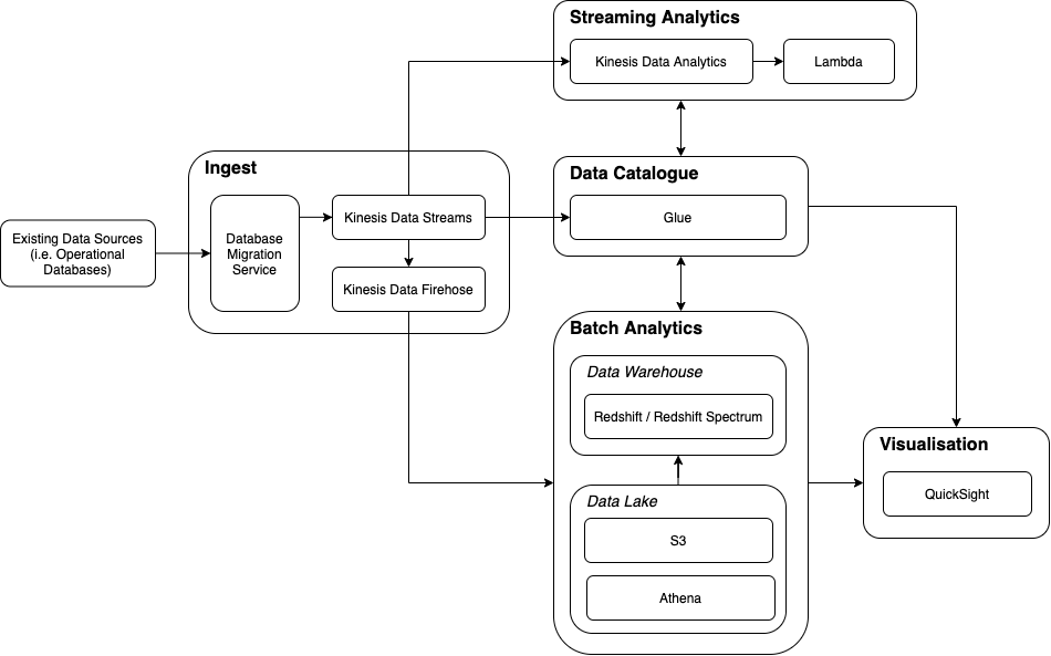
The Data Analytics Reference architecture used by Congo is below:

In summary, this architecture supports the ingest of data into an analytics platform for both batch and stream processing, with support for visualisation. The following sections explain each component of the Reference Architecture followed by an explanation of how AWS products relate to them.
Ingest
It is the role of the Ingest component to bring data into the analytics platform and make it available to the other components – this can be achieved in a number of ways such as:
- Periodically copying entire datasets into the platform (i.e. copy to replace).
- Applying the changes to the analytics platform as and when they happen in the operational database – a technique known as Change Data Capture (CDC).
- Piggy-backing off of existing components such as message streaming architectures to also consume this information.
As part of ingesting data, we may wish to transform it so that it’s in a format the analytics platform can work with.
Once we have data inside the platform, we need to understand it’s format (schema), where it’s located, etc. This is the role of a Data Catalogue.
Data Catalogue
Data Catalogues can be complex systems – their core functionality is to record what datasets exist, their schema and often, connection information – a good example is Kaggle. However, they can be much more complicated offering capabilities such as data previews and data lineage.
Once the catalogue is populated with schemas, it can act as a directory for the rest of the platform to simplify operations such as Query, Visualisation, Extract-Transform-Load (ETL) and access control.
With the data in the platform and its structure understood, we can begin to complete analytical tasks such as Batch Analytics.
Batch Analytics
Batch Analytical processing takes a given defined input, processes it and creates an output. Batch data can take many forms such as CSV, JSON and proprietary database formats. Within a Data Analytics Platform, this data can be stored in two primary ways:
- Raw (i.e. CSV, JSON) – known as a Data Lake
- Processed (i.e. a purpose-built analytics Database) – known as a Data Warehouse
Regardless as to what storage platform we use, what’s common is that a distributed architecture is required to spread the data across compute resources such that queries can be chopped up and executed in parallel as much as possible.
Data Lake
What is meant by processed data? Imagine Congo extract data from their Order Management and CRM systems – at a high-level, the data models of the exported data will look something like:
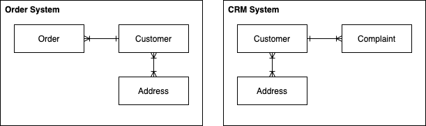
We could take these exports, split them up as outlined earlier, and store them on a number of computers so that we can query them – this is the role of a Data Lake.
When we bring data into an analytics platform, we often want to query across the data so that we can gain insights from data across our organisation. When brining together data from multiple systems, we often end up with duplication (i.e. multiple definitions of a customer), varying data quality, etc. Often we want to process the data to consolidate on a consistent schema and transform incoming data into – we then want to store this data in a single place whereby it can be joined with other data and queried in a straightforward way. This is the role of the Data Warehouse.
Data Warehouse
We can consolidate the 2 data models above into 1 consistent model such as:
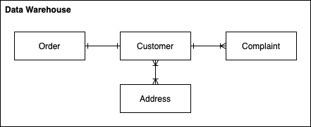
This would be the data model within our Data Warehouse where we’ve merged customer details (perhaps by performing some matching), performed some normalisation and defined relationships between the now common entities. It is much easier to query across 4 concise, defined tables, as opposed to 6 tables containing potentially duplicate data in varying formats.
Data Warehouses come with complexity – often they’re costly and complex to manage. Sometimes we just have large volumes of raw data (i.e. CSVs) that we want to analyse – this is the job of a Data Lake.
Data Warehouses and Data Lakes provide a location within which batch data can be stored and queried, however they’re typically not a great mechanism for reacting to data in realtime – this is the focus of Streaming Analytics.
Streaming Analytics
Unlike Batch Analytics where there is a defined dataset (i.e. we know the number of records), with streaming analytics there is no defined dataset. As such, if we want aggregate data, join data, etc. we must define artificial intervals at within which we perform analytics. For example, Congo want to know what products are hot right now (not the DJ Fresh kind) – ‘now’ could be defined as what’s being doing well over the past 30 minutes. Therefore, as customer orders come in, we might aggregate the quantity purchased for every product over a rolling 30 minute window. At the end of the window, we can use this data to understand what products are hot – perhaps storing the top-10 in a database available to our website so that these products can be shown on the homepage, promoting the sale of those products.
Sometimes we don’t want the results of our analytics to be sent back to another system, sometimes we want to display the results to a data analyst, or perhaps we want to show them the raw data and let them perform the analysis. This is the responsibility of Visualisation.
Visualisation
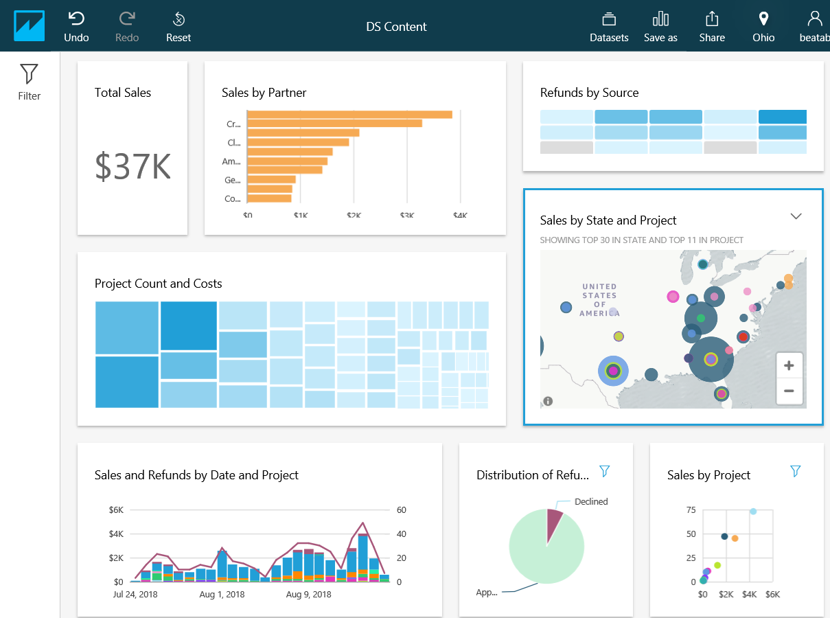
The most basic form of data visualisation is a Table, but as you can see from the image below, tree-maps, geo-maps and charts are all fantastic tools and only touch the surface of what is possible.
This is the end of the Reference Architecture section – now that the cookie-cutters are on the table, we can start making the cookie dough.
Congo Data Analytics on AWS
Congo have decided to implement their Data Analytics Platform in AWS using the Data Analytics Reference Architecture described above. In the diagram below, each component of the Reference Architecture is expanded to include the AWS technologies employed.
The following sections outline the high-level characteristics of each tool.
Ingest
In the Congo implementation, we utilise Kinesis Data Streams as the Ingest ‘buffer’ for data extracted from operational databases using the Database Migration Service.
Database Migration Service
Amazon’s Database Migration Service (DMS) provides a way of moving data from source databases such as Oracle, MySQL, etc. into a number of target locations such as other databases (sometimes referred to a sinks). In Congo’s case, they use DMS to perform an initial full load of the CRM, Order and Product Management systems and subsequently run CDC to feed ongoing changes into the platform. Congo extract all of their data using DMS onto a Kinesis Data Stream.
Kinesis Data Streams
Kinesis Data Streams is a messaging platform – instead of phoning up a friend tell them some news, you put that news on Facebook (i.e. a notice board) for consumption by all of your friends. Messaging systems typically help you decouple your data from its use.
The Database Migration Service will extract data from Congo’s operational systems and put it on the notice board (Kinesis Data Stream). In the diagram below, we can see that 5 ‘records’ have been added to the notice board.

Kinesis Data Streams is AWS’s high-performance, distributed streaming messaging platform allowing messages to be processed by many interested parties at extremely high velocity. For Congo, they provide a single place to make available ingested data for both Batch and Streaming analytics.
Kinesis Firehose
Kinesis Firehose provides a mechanism for easily moving data from a Kinesis Data Stream into a target location. In Congo’s case, we want to move the operational data that is available on a Kinesis Data Stream into the Data Lake & Data Warehouse for batch analytics. Data can either be moved as-is into the target, or it can be transformed prior to migration by a Lambda Function.
You may question how a tool can just move data from A to B. Kinesis Firehose must know what schema (the fields) is present on the Kinesis Data Stream and what the schema of the target is so that it can move the data from A to B in the correct places – this is the role of the Data Catalogue.
Data Catalogue
Glue Data Catalogue
AWS’s Glue Data Catalogue exists to allow easy integration with datasets held on both AWS (i.e. a Kinesis Data Stream) and external to AWS such as an on-premise databases. It is not in the same market as something like Kaggle which is consumer facing, providing data previews, user reviews, etc.
Glue Data Catalogue utilises processes known as Crawlers that can inspect data sources automatically to pull out the entities and attributes found within the datasets. Crawlers exists for database engines, files (i.e. CSVs), and streaming technologies such as Amazon Kinesis.
When it comes to using a tool such as Firehose to move data from a Kinesis Data Stream in a Data Warehouse, knowledge of the schemas can allow for automatic migration (i.e. by matching field names) or GUI based, mapping fields from dataset to another, regardless of field names (i.e. Glue Studio).
Batch Analytics
One of Congo’s use cases is to understand seasonal product trends such that they can improve their marketing strategy. This is achieved through Batch Analytics (analysing a known dataset quantity). Within AWS, Redshift provides Data Warehousing capabilities whilst S3 provides Data Lake capabilities.
Redshift (Data Warehouse)
Redshift is Amazon’s implementation of a Data Warehouse. At a high-level, it feels like a relational database and for all intensive purposes it is; it is exercised through SQL. But there are key differences to ensure query performance on extremely large datasets.
Behind Redshift is a cluster of computers operating in a Distributed Architecture. To distribute the data across these clusters, Redshift provides a number of techniques that will be familiar:
- EVEN – each record will be assigned to a computer in a round-robin fashion (i.e. one after the other)
- KEY – much like the clustering techniques described in this post, records with the same ‘key’ will be stored together on the same computer
- ALL – all data will be stored on all computers
- AUTO – an intelligent mix of all the above depending on the evolution of the data, size of the cluster, query performance, etc.
Whilst AWS provide a managed Data Warehouse solution, this comes at a monetary cost and may be ‘overkill’. In some cases, a Data Lake on S3 is more appropriate and in other cases, a mix of the two.
S3 (Data Lake)
This post will not go into detail about what S3 is, but for simplicities sake you can imagine it to be a file system much like what you find on your laptop – it is a collection of directories and files. As such, unlike the Data Warehouse which will manage the storage of your data for you, with a Data Lake we must split large files inline with the strategies outlined in the Distributed Computing section.
Congo have their Customer & Order information in the Data Warehouse and their Product reference data in the Data Lake (it doesn’t need to be processed prior to query and doesn’t change as much as Customer & Order information).
Athena & Redshift Spectrum (Batch Query)
Once we have data in a Data Warehouse and / or Data Lake, we want to query it. In its simplest form, Redshift is queried via Redshift and S3 is queried via Athena. As the AWS toolset has evolved however, this picture is becoming muddied. If you wanted to query data in your Data Warehouse and join it with data in S3, you could use Redshift Spectrum which allowed for this type of query. However, Athena is now supporting this use case in the other direction. I would not be surprised to see some merging of these toolsets in the near future.
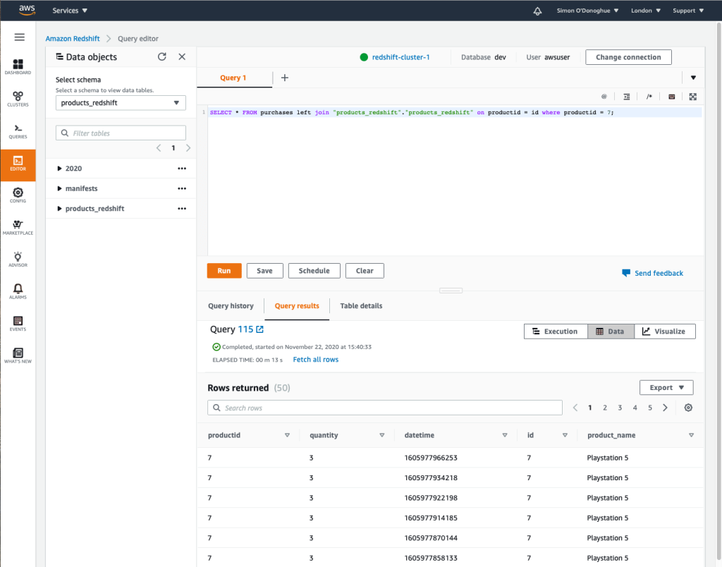
An example of the Redshift Query Editor can be found below – the query is using Redshift Spectrum to join between a table in Redshift and data in an S3 Data Lake.
Both Redshift & Athena support JDBC and ODBC connections and as such, a vast number of tools can send queries to the analytics platform.
This leaves the problem of understanding what products are currently ‘hot’ – for that, we need Streaming Analytics.
Streaming Analytics
We previously discussed Kinesis Data Streams in its role as Ingest for Batch Analytics, but we can also use it as a source for Streaming Analytics and answer Congo’s ‘what’s hot right now?’ question.
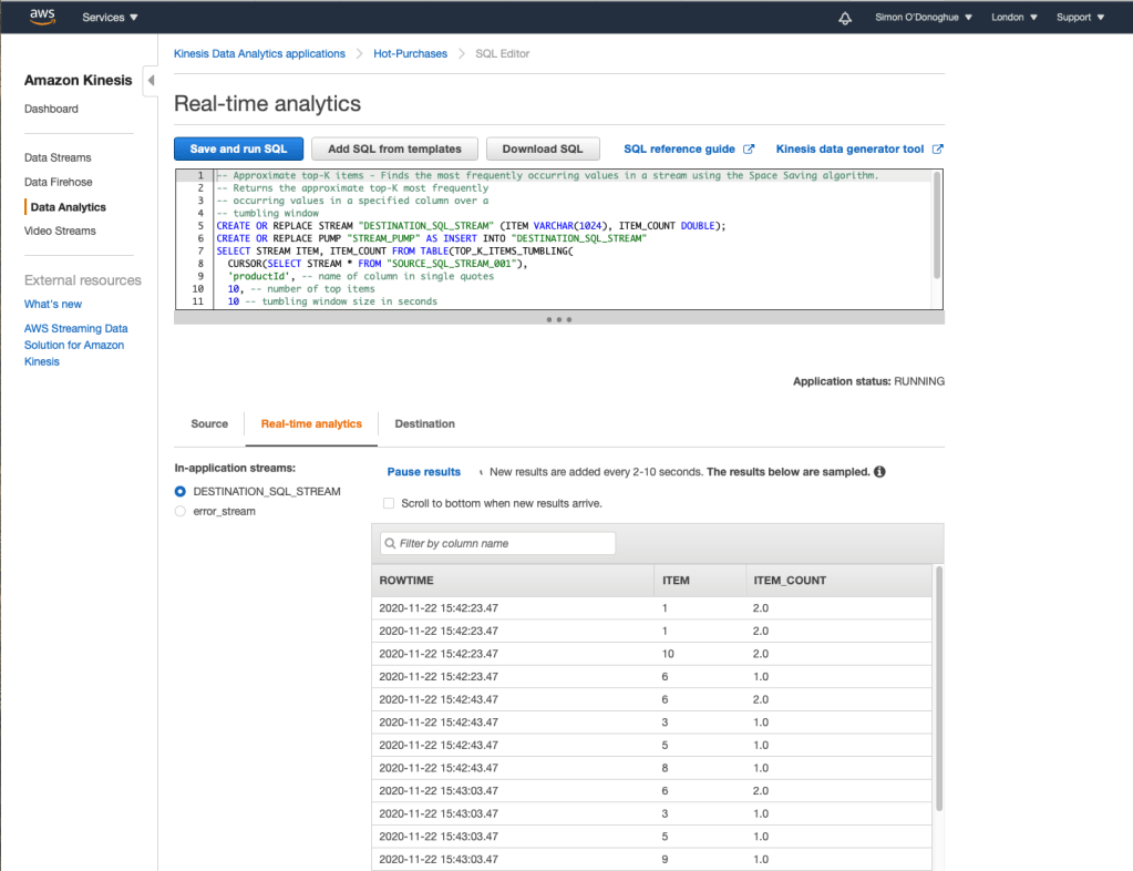
Kinesis Data Analytics (Streaming Query)
Kinesis Data Analytics can be thought of as SQL with Streaming Extensions. Kinesis Data Analytics can buffer based on defined windows, execute the analysis and push the output to a target system.
The query below is utilising a window of 20 seconds to determine the top-K (10) products sold within the window.
What can we do with the results of this streaming analysis?
Lambda
Kinesis Data Analytics can publish the results of the analytics to a number of locations including AWS Lambda – this allows us to essentially do what we like. For Congo, we want to make this analysis available to the Congo website so that hot products can be featured on the homepage – as such, we could publish these results back into an on-premise database accessible to the website.
Visualisation
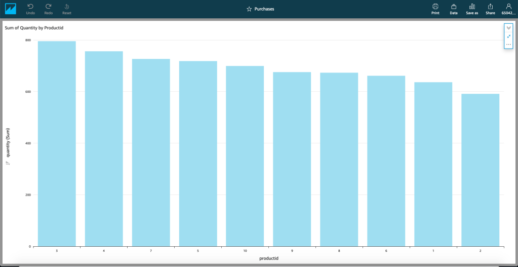
Finally, visualisation. Sometimes the best analysis is performed by humans when given tools that allow the to slice and dice the data as we see fit – AWS QuickSight provides this capability.
QuickSight
QuickSight provides a more typical MI/BI interface such as those found in tools like Microsoft PowerBI – it makes querying your data more accessible than via direct SQL (i.e. makes your data accessible to non-technical resources) and more presentable than a simple table.
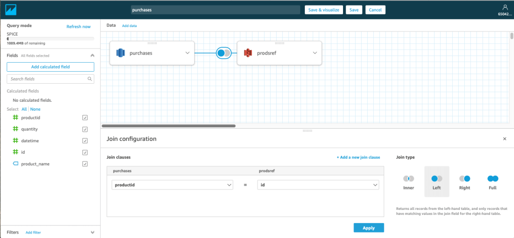
These datasets don’t have to be visualised independently, a table in Redshift can be joined to a dataset in S3 and an on-premise Oracle RDMBS. Through the use of the Glue Data Catalogue, joins can be made through a simple GUI.
But there’s more…
Data Analytics is a huge topic and there are an endless number of tools in the toolbox. AWS itself has much more than discussed in this post such as Neptune for Graph Analytics, EMR for Hadoop ecosystems, Data Pipeline for ETL, Managed Service Kafka (MSK) for long-term distributed streaming, ElasticSearch Service for search and SageMaker for machine learning.
Outside of AWS you have Data Analytics platforms offered by the likes Oracle and Cloudera. One of the main benefits AWS brings to Data Analytics is the massively simplified management – managing a 20 node Apache Hadoop cluster is not easy and finding the people with the skills to do so is equally as challenging. AWS removes this complexity, at a cost.
